
Introduction
Have you ever wanted to draw a smooth curve through your scattered data points? Python's numpy.polyfit allows you to fit a polynomial of any degree to your data using the least squares method. This blog post will explain polyfit in detail, provide interactive examples, and show how to find the best polynomial degree for your data.
1. What is numpy.polyfit?
The function numpy.polyfit(x, y, deg) fits a polynomial of degree deg to the points (x[i], y[i]). It returns the coefficients of the polynomial in decreasing powers.
import numpy as np

x = np.array([1, 2, 3, 4, 5])
y = np.array([2, 4.1, 6.2, 8, 10.1])

# Linear fit
coeffs = np.polyfit(x, y, 1)
print(coeffs)  # Output: [2.02, -0.06]
The result [2.02, -0.06] represents the line y ≈ 2.02x - 0.06.
2. Visualizing Polynomial Fit
You can visualize polynomial fitting using matplotlib and adjust the degree with a slider.
import numpy as np
import matplotlib.pyplot as plt
from matplotlib.widgets import Slider

x = np.array([1,2,3,4,5])
y = np.array([2,4.1,6.2,8,10.1])

def poly_fit_and_mse(x, y, degree):
    coeffs = np.polyfit(x, y, degree)
    p = np.poly1d(coeffs)
    mse = np.mean((y - p(x))**2)
    return p, mse

fig, ax = plt.subplots()
plt.subplots_adjust(bottom=0.25)
degree_init = 1
p, mse = poly_fit_and_mse(x, y, degree_init)
line, = ax.plot(x, p(x), color='blue', label=f'Degree {degree_init}, MSE={mse:.3f}')
scatter = ax.scatter(x, y, color='red', label='Data Points')
ax.legend()
ax.set_title("Polynomial Fit with Adjustable Degree")

ax_degree = plt.axes([0.25, 0.1, 0.65, 0.03])
slider_degree = Slider(ax_degree, 'Degree', 1, 10, valinit=degree_init, valstep=1)

def update(val):
    degree = int(slider_degree.val)
    p, mse = poly_fit_and_mse(x, y, degree)
    line.set_ydata(p(x))
    line.set_label(f'Degree {degree}, MSE={mse:.3f}')
    ax.legend()
    fig.canvas.draw_idle()

slider_degree.on_changed(update)
plt.show()
This interactive plot lets you slide through polynomial degrees and see the curve change dynamically along with the MSE.
3. Finding the Best Degree Automatically
Sometimes, we want Python to select the degree that best fits our data. We can do this by computing the mean squared error for degrees 1 to 10 and selecting the one with the lowest error.
best_degree = 1
min_mse = float('inf')

for deg in range(1, 11):
    _, mse = poly_fit_and_mse(x, y, deg)
    if mse < min_mse:
        min_mse = mse
        best_degree = deg

print(f"Best degree fit: {best_degree} with MSE={min_mse:.3f}")
Python will automatically tell you which polynomial degree best models your data.
4. Key Tips
- Start with low-degree polynomials to avoid overfitting.
- Use weights if some data points are more important.
- Use
numpy.poly1dto make a callable polynomial function. - Visualize the fit to understand how well the polynomial represents your data.
5. Summary
numpy.polyfit is a powerful tool for curve fitting. With sliders, you can make your analysis interactive, and using MSE, you can objectively determine the best polynomial degree. Combine visualization and automatic fitting to make your data analysis both accurate and engaging.


0 Comments